原始感知机算法实现
李航老师《统计学习方法》第二章笔记。 关于原始感知机学习算法的简单实现
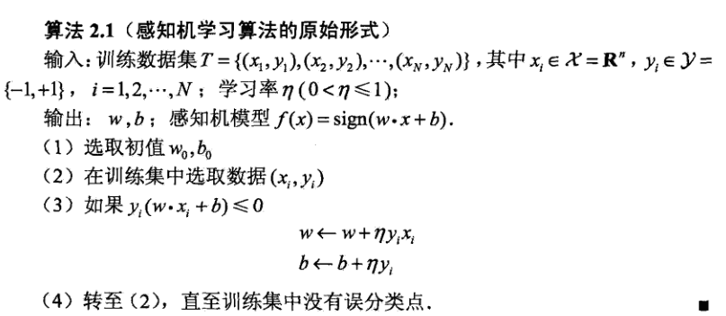
算法原理
算法实现
import numpy as np
from matplotlib import pyplot as plt
# S1-->随机生成训练集并标注
# train matrix
def get_train_data():
M1 = np.random.random((100, 2))
M11 = np.column_stack((M1, np.ones(100)))
M2 = np.random.random((100, 2)) - 0.7
M22 = np.column_stack((M2, np.ones(100) * (-1)))
MA = np.vstack((M11, M22))
plt.plot(M1[:, 0], M1[:, 1], 'ro')
plt.plot(M2[:, 0], M2[:, 1], 'go')
min_x = np.min(M2)
max_x = np.max(M1)
# 此处返回 x 是为了之后作图方便
x = np.linspace(min_x, max_x, 100)
return MA, x
# S2-->原始感知机模型的训练及做图
# 感知机模型:f(x) = sign(w*x+b)
def func(w, b, xi, yi):
num = yi * (np.dot(w, xi) + b)
return num
# 训练 training data
def train(MA, w, b):
# M 存储每次处理后依旧处于误分类的原始数据
M = []
for sample in MA:
xi = sample[0:2]
yi = sample[-1]
# 如果为误分类,更新 w, b
# n 为学习率
if func(w, b, xi, yi) <= 0:
w += n * yi * xi
b += n * yi
M.append(sample)
if len(M) > 0:
train(M, w, b)
return w, b
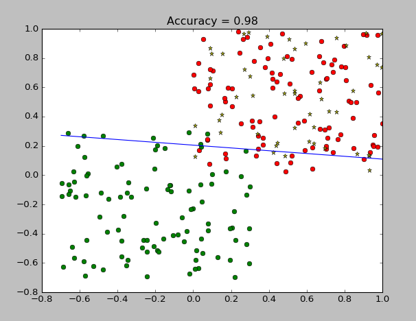
# 作出分类线的图
def plot_classify(w, b, x, rate0):
y = (w[0] * x + b) / ((-1) * w[1])
plt.plot(x, y)
plt.title('Accuracy = ' + str(rate0))
# S3-->随机生成测试集,并测试模型
# 随机生成 testing data 并作图
def get_test_data():
M = np.random.random((50, 2))
plt.plot(M[:, 0], M[:, 1], '*y')
return M
# 对传入的 testing data 的单个样本进行分类
def classify(w, b, test_i):
if np.sign(np.dot(w, test_i) + b) == 1:
return 1
else:
return 0
# 测试数据,返回正确率
def test(w, b, test_data):
right_count = 0
for test_i in test_data:
classx = classify(w, b, test_i)
if classx == 1:
right_count += 1
rate = right_count / len(test_data)
return rate
def plot_n_rate(rate_l):
# plot n-rate
n_l = sorted([float(x) for x in rate_l.keys()])
y = [float(rate_l[n_l[i]]) for i in range(len(n_l))]
print(n_l, '\n', y)
plt.plot(n_l, y, 'ro-')
plt.title("n-accuracy")
plt.show()
if __name__ == "__main__":
MA, x = get_train_data()
test_data = get_test_data()
# 定义初始的 w,b
w = [0, 0]
b = 0
# 初始化最优的正确率
rate0 = 0
# rate_l 记录学习率的更新
rate_l = {}
# 循环不同的学习率 n,寻求最优的学习率,即最终的 rate0
# w0,b0 为对应的最优参数
for i in np.linspace(0.01, 1, 1000):
n = i
w, b = train(MA, w, b)
# print(w,b)
rate = test(w, b, test_data)
if rate >= rate0:
rate_l[n] = rate
rate0 = rate
w0 = w
b0 = b
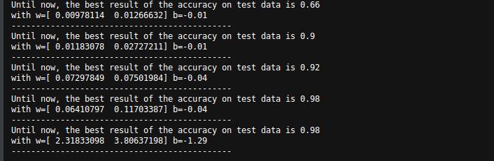
print('Until now, the best result of the accuracy on test data is ' + str(rate))
print('with w=' + str(w0) + ' b=' + str(b0))
print("n=", n)
print('---------------------------------------------')
# 在选定最优的学习率后,作图
plot_classify(w0, b0, x, rate0)
plt.show()
# 作出学习率——准确率的图
plot_n_rate(rate_l)
输出: